Examples

Every code block on this page is executed when the documentation is built, so the output shown is real.

A complete example

The full workflow on a smooth four-well objective — approximate, find every critical point, then keep the minima:

using Globtim, DynamicPolynomials, HomotopyContinuation

# Four-well objective: global minima at (±1, ±1), a maximum at the origin, four saddles.
f(x) = (x[1]^2 - 1)^2 + (x[2]^2 - 1)^2

TR  = TestInput(f, dim=2, center=[0.0, 0.0], sample_range=1.5)   # search box [-1.5, 1.5]²
pol = Constructor(TR, 8)                                          # degree-8 Chebyshev fit

@polyvar x[1:2]
sols = solve_polynomial_system(x, pol)                           # solve ∇p = 0
df   = process_crit_pts(sols, f, TR)                             # → true critical points of f
df_enhanced, df_min = analyze_critical_points(f, df, TR; enable_hessian = true, verbose = false)

println("L² approximation error : ", round(pol.nrm, sigdigits = 3))
println("critical points found  : ", size(df, 1))
println("minima found           : ", size(df_min, 1))

L² approximation error : 2.3e-15
critical points found  : 9
minima found           : 4

Degree 8 recovers this quartic essentially exactly (pol.nrm ≈ 1e-15), and Globtim finds all nine critical points — the four global minima at (±1, ±1), plus four saddles and the central maximum. The recovered minima:

using DataFrames   # nrow/eachrow come from DataFrames, which analyze_critical_points returns
sort!(df_min, [:x1, :x2])
[(round(r.x1, digits = 3), round(r.x2, digits = 3)) for r in eachrow(df_min)]

4-element Vector{Tuple{Float64, Float64}}:
 (-1.0, -1.0)
 (-1.0, 1.0)
 (1.0, -1.0)
 (1.0, 1.0)

Runnable demo scripts

Self-contained scripts ship in the examples/ directory. Run any of them from a project that has Globtim installed (e.g. julia examples/custom_function_demo.jl):

For an end-to-end tour across the whole package family (find → refine → plot), see the Ecosystem Walkthrough.

Custom objectives

Any function that accepts a vector x and returns a scalar works. Here a tilted double-well finds its two minima:

using Globtim, DynamicPolynomials, HomotopyContinuation

g(x) = (x[1]^2 - 1)^2 + x[2]^2 + 0.3 * x[1]   # tilt breaks the symmetry between the wells
TR = TestInput(g, dim = 2, center = [0.0, 0.0], sample_range = 1.5)
pol = Constructor(TR, 8)
@polyvar x[1:2]
df = process_crit_pts(solve_polynomial_system(x, pol), g, TR)
_, df_min = analyze_critical_points(g, df, TR; enable_hessian = true, verbose = false)
println("minima: ", size(df_min, 1), "  (global at the deeper, tilted-down well)")

minima: 2  (global at the deeper, tilted-down well)

1D functions with scalar input

For dim = 1, Globtim accepts ordinary scalar functions (sin, cos, …):

using Globtim, DynamicPolynomials, HomotopyContinuation

f = x -> sin(3x) + 0.1x^2
TR = TestInput(f, dim = 1, center = [0.0], sample_range = Float64(π))
pol = Constructor(TR, 12)
@polyvar x[1:1]
df = process_crit_pts(solve_polynomial_system(x, pol), f, TR)
_, df_min = analyze_critical_points(f, df, TR; enable_hessian = true, verbose = false)
println("critical points: ", size(df, 1), "   minima: ", size(df_min, 1))

[ Info:   🚀 lambda_vandermonde_original: Using OPTIMIZED recurrence (Float type)
┌ Warning: Gradient computation failed for 6/6 points
│   failed_points =
│    5-element Vector{Int64}:
│     1
│     2
│     ⋮
│     5
│   error_types =
│    1-element Vector{String}:
│     "MethodError"
└ @ Globtim ~/work/Globtim.jl/Globtim.jl/src/refine.jl:167
┌ Warning: Hessian computation failed for 6/6 points
│   failed_points =
│    5-element Vector{Int64}:
│     1
│     2
│     ⋮
│     5
│   error_types =
│    1-element Vector{String}:
│     "MethodError"
└ @ Globtim ~/work/Globtim.jl/Globtim.jl/src/hessian_analysis.jl:48
critical points: 6   minima: 0

Domain size matters

Globtim finds the critical points inside the search box. Widen the box to capture more of them, and use a rectangular box (sample_range as a vector) for anisotropic domains:

TR = TestInput(f, dim = 2, center = [0.0, 0.0], sample_range = 1.5)        # square [-1.5, 1.5]²
TR = TestInput(f, dim = 2, center = [0.0, 0.0], sample_range = [2.0, 1.0]) # rectangle [-2,2]×[-1,1]

High-dimensional problems (3D / 4D)

The same workflow scales to 3D and 4D. Practical tips:

• Reduce the polynomial degree as dimension grows (4D → degree 4–6 is often enough for smooth objectives).
• Use precision = AdaptivePrecision when you need higher-accuracy coefficients (e.g. for sparsification or the symbolic solver).
• Pass enable_hessian = false to analyze_critical_points for a faster pass when you only need the minima.

See high_dimensional_demo.jl for a worked 3D/4D scaling example.

Visualization

Plotting the polynomial level set with critical points overlaid lives in the GlobtimPlots package. Load a Makie backend (CairoMakie for static files, GLMakie for interactive windows) before calling any plot function:

using GlobtimPlots, CairoMakie

apol = adapt_polynomial_data(pol)    # adapt Globtim objects for plotting
ainp = adapt_problem_input(TR)
fig  = cairo_plot_polyapprox_levelset(apol, ainp, df_enhanced, df_min)
CairoMakie.save("levelset.png", fig)

See the GlobtimPlots repository for the full set of plot types (Morse spectra, subdivision partitions, convergence sweeps).

Statistical analysis and tables

Enhanced statistics and CSV / Markdown / LaTeX table export live in GlobtimPostProcessing, which consumes the df_enhanced DataFrame produced above:

using GlobtimPostProcessing
export_analysis_tables(tables, "critical_point_analysis", output_dir; formats = [:csv, :markdown, :latex])

Test-function gallery

Globtim on the Deuflhard test function — sample grid, polynomial approximant, and recovered minima:

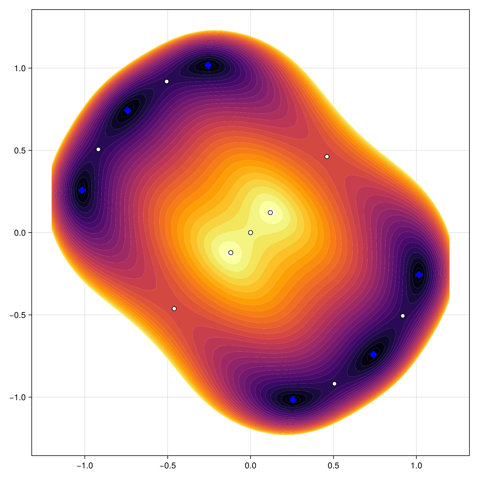
More benchmark objectives (Beale, Branin, Hölder Table, …) are available as built-in test functions; see the FUNCTION_REGISTRY and examples/ scripts to reproduce them.

Next steps

• Getting Started — basic concepts and setup
• Core Algorithm — the mathematical approach
• API Reference — the rendered function reference
• Precision — precision types and trade-offs
• Sparsification — polynomial complexity reduction